Monday, November 30, 2015

Energy Conservation

In the days in which General relativity celebrates its first one hundred years (I believe the paper was published Dec 2 1915), I want to talk about energy conservation, which is a topic relevant to general relativity and to hydrology too. 

“One of the founding principle of Thermodynamics is that energy is always conserved. It can be transformed in one form to another, but it is never created or destroyed (but see below). The first principle of Thermodynamics was given something like in its modern form by Robert Mayer (see also here) in the 1840s -shortly before the concept of energy, as we understand it, was introduced into science. Mayer, a German doctor, became intrigued by the observation that the blood  he was letting from the veins of feverous sailors in the Dutch West Indies was considerable redder than he has would expected (read the full story in the Oliver Morton’s book, the entertaining lecture for a hydrologist, I am using here)” … Mayer deduced the the sailors were using less oxygen than expected due to the warmer climate and was brought to the conclusion that respiration in animals was a specialised form of combustion (which was a common, but not universally accepted belief among the chemist’s contemporary to Mayer).  “However, Mayer decided that the total amount of heat generated in the body must be equal to the capacity of generating force latent in food. Mayer was subsequently lead to  look at the sun, and he arrive to argue that sunlight was the sustenance from plants and  these of animals. Plants were converting energy from light to a chemical form.” 
Other famous scientists were subsequently working on energy conservation law, and maybe you associate the law with the name of Joule

Therefore the early discovering of the energy conservation is extraordinarily close to what modern hydrological studies pursue, especially now that the food-climate-water nexus is at the center of entire research programs.  

A famous finding  of Albert Einstein is the equivalence of energy and mass. This looks like an exotic property, but it is actually always present in hydrological thermodynamic: what else is the “latent heat” if not an explicit statement that mass (and forms of its arrangements, the phases) is a form of energy ? 
Since water on earth and in the hydrological cycle changes phase, water energy budget must account for mass transfer.  However, because also mass, besides energy, is conserved,  energy equation  is greatly simplified. 
If mass conservation is given for granted in hydrology (but not always completely accounted for: because people focuses more -erroneously - on the fluxes), energy conservation is rarely considered. Our GEOtop is one of the few models that does it, and considers energy conservation together with mass conservation (and the budgets, not just the flows!) with an appropriate level of complexity.

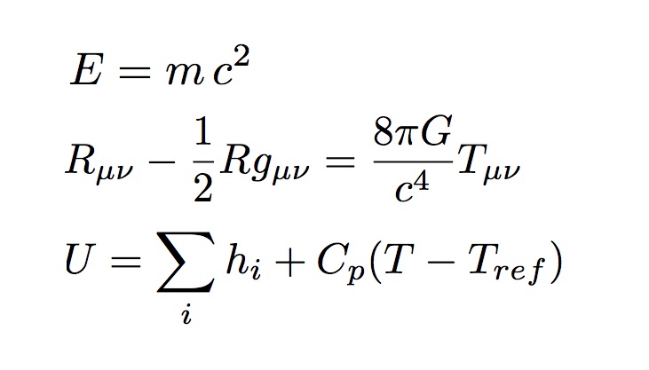
Going back to the main argument, what was an experimental achievement for Mayer, became, after Emmy Noether, a Swiss mathematicians a property connected with the symmetry of the mathematical structure of Mechanics (and Electromechanics indeed) when presented in Lagrangian of Hamiltonian form. Noether’s theorems simply state that if the Lagrangian (Hamiltonian) - either classic or quantistic - of a certain system is invariant under a group of transformations, this implies a conservation law. Energy conservation is, in fact, implied by invariance in time of the Galilean physics, while, for instance, momentum conservation is implied by invariance under space translations (and angular momentum is conserved because of invariance under rotations of the reference frame).  Special relativity does not alter this situation so, in special relativity, mass, energy and momentum are conserved, as well as in Galileian/Newtonian mechanics.  The new ingredient in Special relativity is that space is not separated by time, but both are connected. So, actually the above conservation laws are all connected (and the first of the three equations in the figure says part of it). 

However, the one hundred years old second equation of the figure states that the stress tensors (a sort of generalisation of energy, that compares in the second member of the equation, please see Wikipedia) is strongly connected with the geometry of space. So, at large, energy, mass, time, space, matter are all connected, but energy is not conserved in the Universe (and BTW also some arguments about the thermodynamical death of the University are not very solid).  Please find a more detailed and technical explanation here; another explanation here

Energy is conserved on earth, with great precision (for a Hamiltonian treatment of Earth's fluid mechanics, please refer to the Salmon book, or his paper), and studying the arrangements of matter is important in hydrology. For us it is an approximation that works, and it is very stupid not to use it. 
When accounting for it obviously we have to deal with both kinetic and potential energy, but also internal energy has a big role, especially when we arrive to talk how liquid water becomes ice, or water vapour or viceversa, which continuously happens.  The third equation in Figure reminds it, being mass hidden in enthalpies, and in thermal capacity (for general references to Thermodynamics see here). 

The game becomes thermodynamic also for Hydrology and, actually, the third equation just gives a flavour of it, because when phases are involved, also their interfaces  and their mixing must be taken into account: otherwise we do not understand how drops form, or water is retained in vadose soils, or how it freezes, or how flows in plants.

But these are stories for another day.


Thursday, November 26, 2015

Rainfall on the Blue Nile

Assume you want to forecast the discharge and the hydrological cycle of a large African river.  Meteorological stations are just a few in a wide area, and gauge stations too, indeed. So what to do,while attending that more measurements are made ?  Simply you have to use satellite data. This paper, by Abera et al., deals with the analysis of five satellite data and analyse their reliability in the Blue Nile region.
Among the five there is the innovative product by Luca Brocca SM2RAIN which infers precipitations from the soil moisture analysis.
Please find the preprint of the paper under the Figure.  The abstract of the paper reads: 

"In a region where ground-based gauge data are scarce, satellite rainfall estimation (SREs) products are a viable option for proper space-time rainfall characterization. However, their accuracy and performances vary from region to region, and must be assessed. In this study, five high resolution satellite products (TRMM, CMORPH, TAMSAT, SM2R-CCI, and CFSR) are compared and analysed using the available rain gauge data in one of the most topographically and climatologically complex regions, Upper Blue Nile basin. The basin rainfall is investigated systematically, and it is found that, at some locations, the difference in mean annual rainfall estimates between these SREs could be as much up to 2700 mm. Considering three goodness-of-fit indexes, correlation, bias and root mean square error (RMSE) between the SREs and ground-based gauge rainfall, CMORPH, TAMSAT and SM2R-CCI outperform the other two. TAMSAT has the highest (91%) detection skill for dry days, followed by the CFSR (77%). For lower rainfall values, CMORPH, TAMSAT and CFSR show a higher accuracy index than SM2R-CCI and TRMM. On the contrary, the SM2R-CCI has the highest accuracy index for medium rainfall ranges (10-20 mm). In addition to the identification of the best performing products, the study tried to determine the bias correction of the estimates. A confusion matrix is used to investigate the detection ability of satellite rainfall products for different rainfall intensities. The empirical cumulative distribution (ecd f ) mapping technique is used to correct the SREs intensities distribution. This method provides a means to improve the rainfall estimation of all SREs, and the highest improvement obtained is for CMORPH (from -70% to -4%). "

A presentation (here) on the same topics of the paper was given at the 10th Alexander von Humboldt EGU Topical Conference held in Addis Ababa,  this 18-20 November.

The page where the complimentary material for the paper can be found is here.

Tuesday, November 24, 2015

Geomorphological control on variably saturated hillslope hydrology and slope instability

This paper, which has a long history, treats the influence of geomorphology on stability. Not a new topic indeed, but usually saying that convergent topographies favour landslids was a matter of qualitative arguments.  Here it is made by using DEM analysis, a 3D Richards equation solver, and a sound model for hillslope stability. That's the difference for who can appreciate it.
Please, find the preprint, clicking on the Figure. I think the reading is enjoyable and I hope the Journal will accept it soon. 

Thursday, November 19, 2015

How many leaves has a tree ?

Sometimes ago I asked myself how many leaves a tree has (a real tree, not the homonymous informatics structure). Certainly, it depends on the type of tree, the size of the leaves, and the season too. A simplification would probably be to estimate which is the maximum number of leaves a tree can have. The question was raised by the contemplation of woodland in Trentino but also has an impact on hydrology. No leaves, no transpiration, and maybe, more leaves more transpiration, even if as a possibility ( for which hydrologists coined the infamous potential evapotranspiration concept). I started to google around in trying to understand.*

Many internet surfers report this:

It depends on the tree's species and age, but a mature, healthy tree can have 200,000 leaves. During 60 years of life, such a tree would grow and shed 3,600 pounds of leaves, returning about 70% of their nutrients to the soil.

and cite as source the Wisconsins County Forests Association: but, on their site, I was not able to find the cited words. Anyway, anticipating the answers, this number mentioned is in the range most of leaves' counters gives, at the end (did they influences each other?).

I personally found three approaches to solve the problem. 

The first was simply to count the leaves on a tree. Probably some one really did it. But I could not find trace of it.    Some others made it indirectly Here you will find a counting exercise for kids (but that adults can enjoy).  Even a Wired's journalist got this problem to solve. Another version of the same approach is here.

These professor Morrow's students, instead, were actually interested in the weight of leaves (and I can understand they were possibly interested to estimate the gross primary production). These students of Mathematics built actually a model of plant growth. Their interesting trial, which has to do also with fractals, can be found here

The third method is based on determining the leaf area index (LAI, see Baldocchi’s Notes first), the ratio between the surface of the total area of the leaves in a canopy, divided by the projected area the canopy covers. It seems, that under many circumstances this quantity is easier to measure (it can be obtained also from satellites) that counting the the leaves (or is it a modern automatic way to do it ?)
Having the LAI and the canopy area covered by a tree (which is actually very similar to what done in the “counting methods above”) the number of leaves can be estimated, indeed even over large scale. or an entire forest. 

The problem is connected with others like; How big a tree leaf is  or how much it weights. 

See below a short bibliography on the leaf area index and on its implications. 

P.S. - Section 2.3 of G. Bonan 2019 book talks about the leaf mass per unit area and can be partially used to complement this post. 

* This part was edited by Barry Galvin.

Leaf Area Index

Asher G.P, Scurlock J.M.O, Hicke J.E., Global synthesis of leaf are index observations: implications for ecological and remote sensing studies, Global Ecology and Biogeography, 12, 191-205, 2003

Breda N.J, Ground-based measurements of leaf area index: a review of methods, instruments and current controversies, Journal of experimental Botany, 54(392), 2403-2417, 2003

Bonan, Gordon. 2019. Climate Change and Terrestrial Ecosystem Modeling. Cambridge University Press.


Colombo R., Bellingeri D., Pasolini D., Marino C.M., Retrieval of leaf area index in different vegetation types using high resolution data, (Also here) Remote Sensing and Environment, 86, 120-131, 2003


Grier, G.C., Running, S.W., Leaf area of mature northwesternconieferous forests: relation to site water balance, Ecology, 58: pp: 893-899, 1977

Norman, J.M., Campbell G.S., In: Canopy structure, Chapter Plant Physiological Ecology, pp 301-325, Springer-Verlag, 2000,  DOI:10.1007/978-94-010-9013-1_14

Pasolli L, Asam S., Castelli M, Bruzzone L, Wohlfahrt, Zebisch M, Notarnicola C,  Retrieval of Leaf area index in mountain grasslands in the Alps from MODIS satellite images, Remote Sensing of Environment, 159-174, 2015


Wang Q., Adieu S., Tenhunen J, Granier  A., On the relationship of NDVI with leaf area index in a deciduous  forest site, Remote Sensing, 94, 244-255, 2005


Monday, November 16, 2015

Granular Flows in Climaware

Under the name of granular flows are included snow avalanches, debris flows, and sediment generation and transport. CLIMAWARE has a task devoted to them, with application to river Adige.
Colleague Michele Larcher covers the snow avalanches part, and by clicking on the figure below, you will find his presentation of the topic.
This was actually a three parts seminar. The second part, held by Luigi Fraccarollo regarded the suspended sediment in river Adige, and the study of its origin.
The last part was mainly on debris flow and the model Trent2D, an innovative code to estimate them, by Giorgio Rosatti and co-workers (GS).

The challeng is to blend all of this in the unique framework of the project.


Thursday, November 12, 2015

The GEOframe blog

Hoping that the documentation efforts become torrential, I opened a new blog, just dedicated to the documentation of GEOtop and JGrass-NewAGE source code and executables.
The blog is linked in the Related blog banner. Otherwise, you can click here: http://geoframe.blogspot.com.
Geoframe is an idea first envisioned a few years ago, whose general concepts can be found in this presentation given at 2008 CUASHI biennial meeting (the only change to be done is the substitution of OpenMI with OMS).

Wednesday, November 11, 2015

Urban Hydrology

Today, I gave a seminar on perspectives in urban hydrology. The sponsor where two companies producing road paving and infrastructures for sewage systems. The audience was a group of Italian professional, and I try to convey some concepts regarding the integrated water management and how to calculate it.

Slides of the talk are obtained by clicking on the figure above. An interesting post, connected with this presentation comes from Tony Ladson and is entlitled: Does stormwater management works ?

Selected References

Berne, A., Delrieu, G., Creutin, J.-D., & Obled, C. (2004). Temporal and spatial resolution of rainfall measurements required for urban hydrology. Journal of Hydrology, 299(3-4), 166–179. http://doi.org/10.1016/j.jhydrol.2004.08.002

Delleur, J. W. (2003). The Evolution of Urban Hydrology: Past, Present, and Future. J.of Hydraul. Eng., 129(8), 563–573.

Livingston, E. H., & McCaron, E. (2007). STORMWATER MANAGEMENT: a guide for Floridians (pp. 1–72). U.S. Environmental Protection Agency.

Marsalek, J., Jimenez-Cisneros, B. E., Malquist, P. A., Karamouz, M., J, G., & Chocat, B. (2006). Urban water cycle processes and interactions (No. 78) (pp. 1–92). Paris.

Niemczynowicz, J. (1999). Urban hydrology and water management present and future challenges. Urban Water, 1, 1–14.

Ranzato, M., Integrated water design for a decentralized urban landscape, Doctoral School in Environmental Engineering, Trento 2011

Sunday, November 8, 2015

CLIMAWARE project (again) at the Anticipation Conference

Here in Trento, the last three days was organised a Conference on Anticipation promoted by the UNESCO chair on Anticipatory systems. I participate as auditor in one of the sessions, and the experience was, at the same time interesting and different. Interesting and different because, it was disclosing to me the view of economists and sociologists on the topic, and I had to sinchronize my brain on their language and quirks. However, there was also a session on Anticipation in Engineering in which we presented the project CLIMAWARE. Presentation was given by Lavinia Laiti, and I think it gives a consistent overview of the project.

Clicking on the above image, you will have access to the slides view. Enjoy!

Tuesday, November 3, 2015

Climate modelling of Alpine Areas

Our project CLIMAWARE started last May and will endure for the whole 2016. It tries to use climate projections to estimate impacts on water resources, and from there, to ecosystem services and society in general. The scope of the model is very wide, since it aims also to join expertise and people coming from different disciplines. In order to have a unified language inside the group we started a series of talks. The first one was given by Lavinia Laiti,  for the group of Atmospheric Physics of our Department. Here below, clicking on the image, please find her seminar's slides (in Italian). 
For sake of convenience, I report here below the bibliography that was cited. Notably, the same topics were also covered at the Alpine Convention held in September 2014 in Trento. Who is interested can find the slides here

References

Auer et al. (2007): HISTALP - Historical instrumental climatological surface time series of the Greater Alpine Region. Int. J. Climatol., 27, 17- 46. 

Beniston et al. (2007): Future extreme events in European climate - an exploration of regional climate model projections. Climatic Change 81, 71–95. 

Brunetti et al. (2006): Precipitation variability and changes in the greater Alpine region over the 1800-2003 period. J. Geophys. Res., 111, D11107. 

Brunetti et al. (2009): Climate variability and change in the Greater Alpine Region over the last two centuries based on multi-variable analysis. Int J Climatol, 29, 2197-2225. 

Bucchignani et al. (2013). Simulation of the climate of the XX century in the Alpine space. Nat. Hazards, 67, 981–990.

Bucchignani et al. (2015): High-resolution climate simulations with COSMO-CLM over Italy: performance evaluation and climate projections 
for the 21st century. Int. J. Climatol., DOI: 10.1002/joc.4379
Frei et al. (2003). Daily precipitation statistics in regional climate models: Evaluation and intercomparison for the European Alps. J. Geophys. 
Res., 108(D3), 4124.

Frei et al. (2006), Future change of precipitation extremes in Europe: Intercomparison of scenarios from regional climate models, J. 
Geophys. Res., 111, D06105.

Frei and Schär (1998): A precipitation climatology of the Alps from high-resolution rain-gauge observations. Int. J. Climatol., 18, 873-900. Giugliacci et al. (2010). Manuale di Meteorologia, 2nd ed. Alpha Test, 763 pp.

Gobiet et al. (2014): 21st century climate change in the European Alps - A review. Sci. Tot. Env., 493, 1138-1151.

Haslinger et al. (2013). Regional climate modelling over complex terrain: an evaluation study of COSMO-CLM hindcast model runs for the  Greater Alpine Region. Climate Dynamics 40, 511-529.

Haylock et al.(2008): A European daily high-resolution gridded dataset of surface temperature and precipitation for 1950-2006. Journal of Geophysical Research, 113, D20.

Isotta et al. (2014): The climate of daily precipitation in the Alps: development and analysis of a high-resolution grid dataset from pan-Alpine rain-gauge data. Int. J. Climatol., 34, 1657–1675. 

Jacob et al. (2014): EURO-CORDEX: new high-resolution climate change projections for European impact research. Regional Environmental Change, 14, 563-578. 

Kotlarski et al. (2015): The elevation dependency of 21st century European climate change: an RCM ensemble perspective. Int. J. Climatol. Montesarchio et al. (2014): Performance evaluation of high-resolution regional climate simulations in the Alpine space and analysis of 
extreme events, J. Geophys. Res. Atmos.,119.

Philipona (2013): Greenhouse warming and solar brightening in and around the Alps. Int. J. Climatol., 33, 1530-1537.

Prein et al. (2011): Analysis of uncertainty in large scale climate change projections over Europe. Meteorol. Zeit., 20, 383-395.

Prein et al. (2013): Added value of convection permitting seasonal simulations. Clim. Dyn. 41, 2655–2677.

Rajczak et al. (2013). Projections of extreme precipitation events in regional climate simulations for Europe and the Alpine Region, J. Geophys. Res. Atmos., 118, 3610–3626.

Schär et al. (1998): Current Alpine climate. In Cebon P. et al. (eds.), A View from the Alps: Regional Perspectives on Climate Change. MIT Press.

Suklitsch et al. (2011): Error characteristics of high resolution regional climate models over the Alpine area. Climate Dynamics, 37, 377-390. 

Torma et al. (2015), Added value of regional climate modeling over areas characterized by complex terrain—Precipitation over the Alps, J. 
Geophys. Res. Atmos., 120, 3957–3972.

Turco et al. (2013): Assessing gridded observations for daily precipitation extremes in the Alps with a focus on northwest Italy, Nat. Hazards Earth Syst. Sci., 13, 1457-1468. 

Von Hardenberg et al. (2015):Observations and modelling of precipitation and the hydrological cycle: uncertainties and downscaling. Trento, 4 giugno 2015. 

Web

https://climatedataguide.ucar.edu/climate-data 
http://prudence.dmi.dk/ 
http://www.ensembles-eu.org/ 
http://www.cordex.org/